Seaborn Regplot

A regression evaluation examines the associations between unbiased components or predictors and dependent variables or attributes. There are numerous contradictory approaches to evaluating the regression mannequin. In Python, the “seaborn” module methodology referred to as “seaborn.regplot()” plots/attracts the regression plot.

This write-up will ship you with an intensive information on Python “seaborn.regplot()” methodology utilizing the beneath content material:

What’s the “seaborn.regplot()” Methodology in Python?

The “seaborn.regplot()” perform in Python is utilized to plot/create knowledge and a linear regression mannequin match. It’s an axes-level perform, which signifies that it takes an axes object as enter and returns the identical axes object.

Syntax

The syntax of the “seaborn.regplot()” is proven beneath:

Parameters

Within the above syntax:

• The “x” and “y” parameters are the enter variables. They are often strings, collection, or vector arrays. If they’re strings, they need to correspond to column names within the “knowledge” DataFrame.
• The “knowledge” parameter is a DataFrame that incorporates the “x” and “y” parameters.
• The “x_estimator” parameter is a callable perform that accepts a vector and retrieves a scalar. This can be utilized to remodel the “x” earlier than developing the regression mannequin.
• The “x_ci” parameter specifies the boldness intervals for the regression line. The default worth is “None”, that means that no confidence intervals are plotted.
• The “order” attribute determines the order of the polynomial regression mannequin. The default is “1”, which suggests {that a} linear regression mannequin is match.
• The “strong” parameter implies whether or not to make use of a strong regression mannequin. The default worth is “False”, that means a regular linear regression mannequin is match.
• The “ax” parameter is an axes object that can be utilized to specify the axes on which the plot can be drawn. If it isn’t specified, a brand new axes object can be created.
• The opposite optionally available parameters carry out particular duties when handed contained in the “seaborn.regplot()” methodology.

Return Worth

The “seaborn.regplot()” perform returns the axes object on which the plot was created.

Instance 1: Making use of the “seaborn.regplot()” Perform to Create a Regression Plot

The next code demonstrates the “seaborn.regplot()” methodology:

Within the above code:

• The “seaborn” and “matplotlib” modules are imported.
• The “seaborn.load_dataset()” perform is used to import the predefined dataset named “suggestions”.
• The “seaborn.regplot()” perform is used to plot the regression plot. This perform attracts a scatterplot of two parameters, “x” and “y”, together with a linear regression mannequin match. On this case, “x” is “total_bill”, “y” is “tip”, and the “knowledge” parameter specifies the supply dataset to make use of.

Output

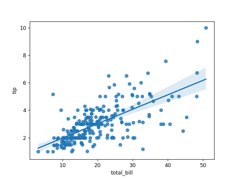
The regression plot has been created primarily based on the above snippet.

Instance 2: Making use of the “seaborn.regplot()” Perform to Create a Regression Plot With Parameters

The beneath code makes use of the “markers” and “colour” parameters to attract the regression plot:

Within the above code strains, the “seaborn.regplot()” perform takes the “colour” and “marker” parameters together with different parameters to attract the regression plot accordingly.

Output

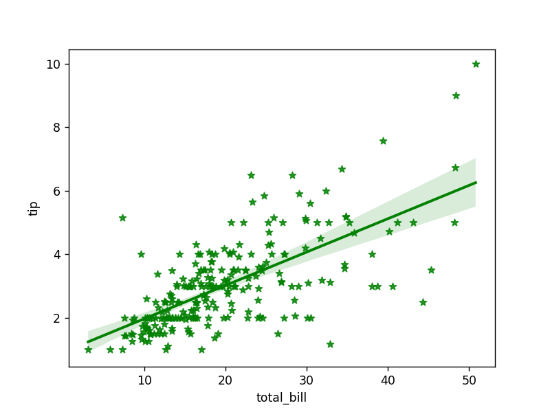
The regression plot has been created.

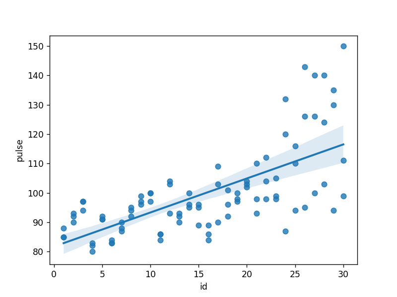
Instance 3: Making use of the “seaborn.regplot()” Perform to a Totally different Dataset

The beneath instance code makes use of the “train” dataset as a substitute and attracts a regression plot:

On this block of code, the “seaborn.load_dataset()” perform takes the “train” dataset as an argument to load the predefined dataset. The “seaborn.regplot()” perform is then utilized to plot the regression plot primarily based on the values of the handed parameters.

Output

Conclusion

In Python, the “seaborn.regplot()” methodology of the “seaborn” module takes the “Datasets” and attracts/constructs the regression plot. On this article, we utilized the “seaborn.regplot()” methodology on numerous predefined datasets resembling “suggestions” and “train” to attract the regression plot. This weblog offered an in depth information on Python’s “seaborn.regplot()” methodology utilizing acceptable examples.