“KDE” plots are much like histograms in how they visualize a dataset’s observations. As an alternative of counting the frequencies of values utilizing bins, “KDE” makes use of a easy curve that represents the likelihood density operate of the variable. By doing this, the distribution’s form and traits may be extra precisely revealed.
This Python publish presents a complete information on the Seaborn “kdeplot()” methodology utilizing quite a few examples:
What’s the Seaborn “kdeplot()” Technique in Python?
The Seaborn “kdeplot()” methodology plots the KDE of a steady variable on a graph. It may be used to visualise univariate or bivariate distributions, in addition to conditional distributions based mostly on a 3rd variable. It will also be used to create “joint”, “marginal”, “rug”, and “contour” plots.
Syntax
seaborn.kdeplot(x=None, *, y=None, vertical=False, palette=None, **kwargs,….)
The Seaborn “kdeplot()” methodology accepts a number of specified arguments that management varied facets of the plot. This methodology retrieves an axis object with the “KDE” plot displayed.
Instance 1: Making a Easy Univariate KDE Plot
On this instance, we’ll create a easy univariate “KDE” plot using the Seaborn “kdeplot()” methodology:
import seaborn as sb
import numpy
from matplotlib import pyplot as plt
knowledge = numpy.random.regular(measurement=1000)
sb.kdeplot(knowledge, shade=‘pink’, fill=‘True’)
plt.present()
Within the above code:
- The “seaborn”, “numpy” and “matplotlib” libraries are imported at the beginning, respectively.
- The “random.regular()” operate is used to create some random knowledge.
- Lastly, the “kdeplot()” methodology is utilized to plot the “KDE” curve for this knowledge based mostly on the desired parameters.
Output
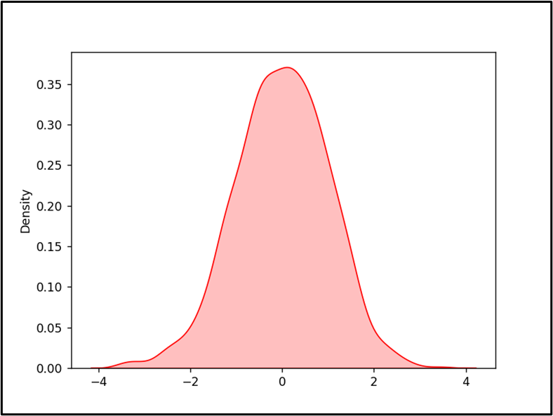
Within the above output, the KDE graph has been displayed in accordance with the desired parameters efficiently.
Observe: The above graph may be inverted utilizing the “vertical=True” parameter within the “seaborn.kdeplot()” methodology.
Instance 2: Making a Advanced KDE Plot With A number of Parameters
The under code is used to plot a multivariate regression “KDE” plot utilizing the “kdeplot()” methodology:
import seaborn as sb
import numpy
from matplotlib import pyplot as plt
knowledge = numpy.random.randn(1000)
data1 = numpy.random.randn(1000)
sb.kdeplot(x=knowledge, y=data1, shade=‘pink’, fill=‘True’, linewidth=3)
plt.present()
On this code:
- The “random.randn()” operate is used to create a numpy array of “1000” random numbers and assign them to the variable “knowledge” and “data1”, respectively.
- These variables are thought of the datasets for the “x-axis” and “y-axis”.
- Now, the “kdeplot()” methodology is used to create a kernel density estimate (KDE) plot of the given two variables “knowledge” and “data1”.
- The KDE plot parameters “shade”, “fill” and “linewidth” are used to customise the kernel density estimate (KDE) plot, respectively.
Output
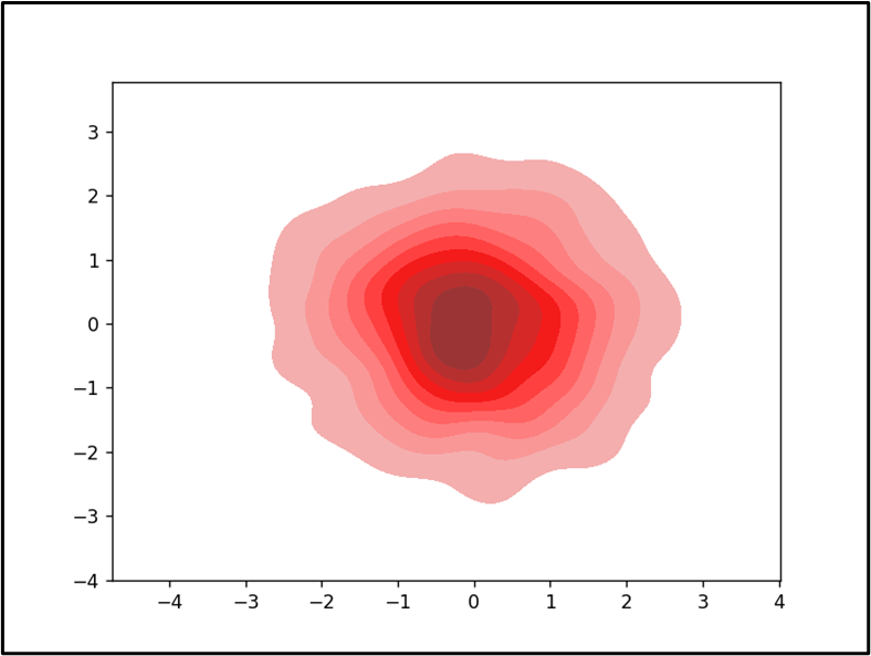
On this final result, the multivariate regression “KDE” plot has been displayed appropriately.
Conclusion
The “kdeplot()” methodology in Python is used to create “KDE” plots that present the distribution of steady variables in a number of dimensions. This methodology can be utilized to create a easy in addition to advanced “KDE” plot with completely different parameters. This methodology additionally helps to visualise and analyze the info, in addition to to check and check completely different fashions. This text defined using the Seaborn “kdeplot()” methodology in Python.