Plotting a number of capabilities in MATLAB gives a robust device for visualizing and evaluating mathematical relationships inside a single graph. Whether or not you’re analyzing knowledge or exploring mathematical ideas, MATLAB provides numerous strategies to plot a number of capabilities effectively. On this article, we’ll discover totally different methods and code examples to plot a number of capabilities in MATLAB, empowering you to create informative and visually interesting plots.
How To Plot A number of Features in MATLAB
Plotting a number of capabilities in MATLAB is critical because it permits for visible comparability and evaluation of various mathematical relationships inside a single graph, enabling insights into their habits and interactions. Under are some frequent methods to plot a number of capabilities in MATLAB:
Technique 1: Plot A number of Features in MATLAB utilizing Sequential Plotting
One simple strategy is to plot every operate sequentially utilizing a number of plot() instructions, right here is an instance:
% Calculate the y-values for every operate
f = sin(x);
g = cos(x);
% Plot every operate sequentially
plot(x, f, ‘r-‘, ‘LineWidth’, 2); % Plots f(x) in crimson with a stable line
maintain on; % Permits for overlaying subsequent plots
plot(x, g, ‘b–‘, ‘LineWidth’, 2); % Plots g(x) in blue with a dashed line
maintain off; % Ends the overlaying of plots
% Add labels and title
xlabel(‘x’);
ylabel(‘y’);
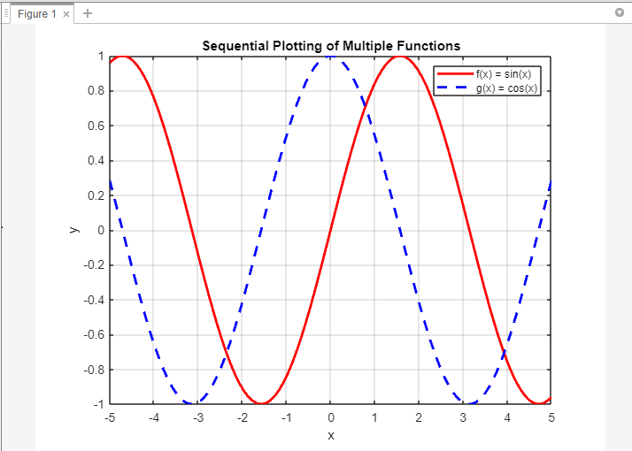
title(‘Sequential Plotting of A number of Features’);
% Add a legend
legend(‘f(x) = sin(x)’, ‘g(x) = cos(x)’);
% Show the grid
grid on;
The code first defines the x-values utilizing linspace() to create a variety of values from -5 to five with 100 factors. The y-values for 2 capabilities, f(x) = sin(x) and g(x) = cos(x), are then calculated utilizing the corresponding mathematical expressions.
Subsequent, the capabilities are plotted sequentially utilizing the plot() operate. The primary plot() command plots f(x) in crimson with a stable line, whereas the second plot() command plots g(x) in blue with a dashed line. The maintain on and maintain off instructions are used to overlay subsequent plots with out clearing the earlier ones.
Technique 2: Plot A number of Features in MATLAB utilizing Vectorized Plotting
MATLAB’s vectorized operations enable plotting a number of capabilities utilizing a single plot() command by combining the x-values and corresponding y-values into matrices. Right here’s an instance:
% Calculate the y-values for every operate
f = sin(x);
g = cos(x);
% Mix x-values and y-values into matrices
xy1 = [x; f];
xy2 = [x; g];
% Plot a number of capabilities utilizing vectorized plotting
plot(xy1(1,:), xy1(2,:), ‘r-‘, ‘LineWidth’, 2); % Plots f(x) in crimson with a stable line
maintain on; % Permits for overlaying subsequent plots
plot(xy2(1,:), xy2(2,:), ‘b–‘, ‘LineWidth’, 2); % Plots g(x) in blue with a dashed line
maintain off; % Ends the overlaying of plots
% Add labels and title
xlabel(‘x’);
ylabel(‘y’);
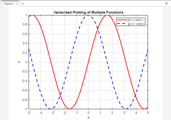
title(‘Vectorized Plotting of A number of Features’);
% Add a legend
legend(‘f(x) = sin(x)’, ‘g(x) = cos(x)’);
% Show the grid
grid on;
The code first defines the x-values utilizing linspace() to create a variety of values from -5 to five with 100 factors.
Subsequent, the y-values for 2 capabilities, f(x) = sin(x) and g(x) = cos(x), are calculated utilizing the corresponding mathematical expressions. These x-values and y-values are then mixed into matrices, xy1, and xy2, the place every matrix consists of two rows: the primary row represents the x-values and the second row represents the corresponding y-values.
Utilizing vectorized plotting, the plot() operate is used to plot a number of capabilities. The primary plot() command plots f(x) by extracting the x-values from xy1(1,:) and the y-values from xy1(2,:), utilizing a crimson stable line. The second plot() command plots g(x) by extracting the x-values from xy2(1,:) and the y-values from xy2(2,:), utilizing a blue dashed line.
Technique 3: Plot A number of Features in MATLAB utilizing Perform Handles
One other strategy entails defining operate handles for every operate and utilizing a loop to plot them. Right here’s an instance:
% Outline operate handles for every operate
capabilities = {@(x) sin(x), @(x) cos(x)};
% Plot a number of capabilities utilizing operate handles
maintain on; % Permits for overlaying subsequent plots
for i = 1:size(capabilities)
plot(x, capabilities{i}(x), ‘LineWidth’, 2); % Plots every operate
finish
maintain off; % Ends the overlaying of plots
% Add labels and title
xlabel(‘x’);
ylabel(‘y’);
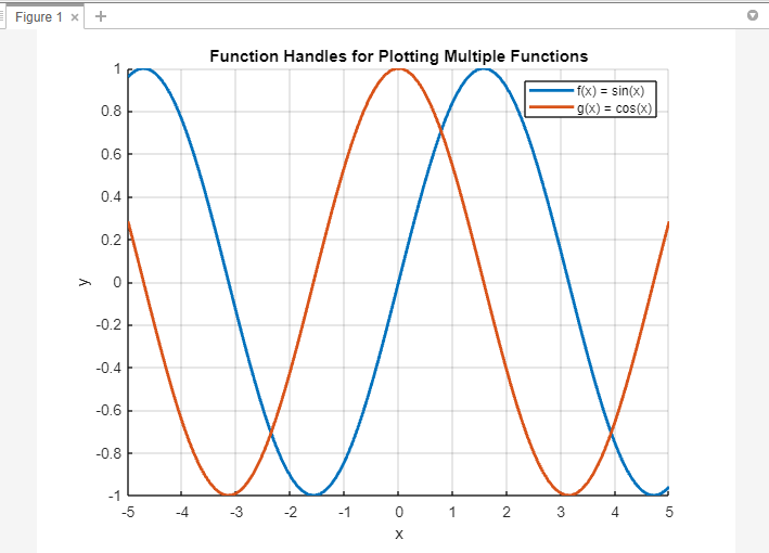
title(‘Perform Handles for Plotting A number of Features’);
% Add a legend
legend(‘f(x) = sin(x)’, ‘g(x) = cos(x)’);
% Show the grid
grid on;
The code first defines the x-values utilizing linspace() to create a variety of values from -5 to five with 100 factors.
Subsequent, operate handles are outlined for every operate utilizing the @() notation. The capabilities variable is an array that holds the operate handles for f(x) = sin(x) and g(x) = cos(x).
Utilizing a loop, the code iterates by every operate deal with within the capabilities array and plots the corresponding operate utilizing the plot() operate. The x-values are fixed for all capabilities, whereas the y-values are obtained by evaluating every operate deal with with the x-values as enter.
The maintain on command permits for overlaying subsequent plots with out clearing the earlier ones. After plotting all of the capabilities, the maintain off command ends the overlaying of plots.
Conclusion
MATLAB gives a number of versatile approaches to plot a number of capabilities, providing flexibility and management over your visualizations. Whether or not you like sequential plotting, vectorized operations, or operate handles, every technique permits you to successfully evaluate and analyze mathematical relationships inside a single graph.